56. Job Search VII: On-the-Job Search#
GPU
This lecture was built using a machine with access to a GPU — although it will also run without one.
Google Colab has a free tier with GPUs that you can access as follows:
Click on the “play” icon top right
Select Colab
Set the runtime environment to include a GPU
56.1. Overview#
In this section, we solve a simple on-the-job search model
based on [Ljungqvist and Sargent, 2018], exercise 6.18, and [Jovanovic, 1979]
Let’s start with some imports:
from typing import NamedTuple

import matplotlib.pyplot as plt
import scipy.stats as stats
import jax
import jax.numpy as jnp
import jax.random as jr
56.1.1. Model Features#
job-specific human capital accumulation combined with on-the-job search
infinite-horizon dynamic programming with one state variable and two controls
56.2. Model#
Let \(x_t\) denote the time-\(t\) job-specific human capital of a worker employed at a given firm and let \(w_t\) denote current wages.
Let \(w_t = x_t(1 - s_t - \phi_t)\), where
\(\phi_t\) is investment in job-specific human capital for the current role and
\(s_t\) is search effort, devoted to obtaining new offers from other firms.
For as long as the worker remains in the current job, evolution of \(\{x_t\}\) is given by \(x_{t+1} = g(x_t, \phi_t)\).
When search effort at \(t\) is \(s_t\), the worker receives a new job offer with probability \(\pi(s_t) \in [0, 1]\).
The value of the offer, measured in job-specific human capital, is \(u_{t+1}\), where \(\{u_t\}\) is IID with common distribution \(f\).
The worker can reject the current offer and continue with existing job.
Hence \(x_{t+1} = u_{t+1}\) if he/she accepts and \(x_{t+1} = g(x_t, \phi_t)\) otherwise.
Let \(b_{t+1} \in \{0,1\}\) be a binary random variable, where \(b_{t+1} = 1\) indicates that the worker receives an offer at the end of time \(t\).
We can write
Agent’s objective: maximize expected discounted sum of wages via controls \(\{s_t\}\) and \(\{\phi_t\}\).
Taking the expectation of \(v(x_{t+1})\) and using (56.1), the Bellman equation for this problem can be written as
Here nonnegativity of \(s\) and \(\phi\) is understood, while \(a \vee b := \max\{a, b\}\).
56.2.1. Parameterization#
In the implementation below, we will focus on the parameterization
with default parameter values
\(A = 1.4\)
\(\alpha = 0.6\)
\(\beta = 0.96\)
The \(\text{Beta}(2,2)\) distribution is supported on \((0,1)\) - it has a unimodal, symmetric density peaked at 0.5.
56.2.2. Back-of-the-Envelope Calculations#
Before we solve the model, let’s make some quick calculations that provide intuition on what the solution should look like.
To begin, observe that the worker has two instruments to build capital and hence wages:
invest in capital specific to the current job via \(\phi\)
search for a new job with better job-specific capital match via \(s\)
Since wages are \(x (1 - s - \phi)\), marginal cost of investment via either \(\phi\) or \(s\) is identical.
Our risk-neutral worker should focus on whatever instrument has the highest expected return.
The relative expected return will depend on \(x\).
For example, suppose first that \(x = 0.05\)
If \(s=1\) and \(\phi = 0\), then since \(g(x,\phi) = 0\), taking expectations of (56.1) gives expected next period capital equal to \(\pi(s) \mathbb{E} u = \mathbb{E} u = 0.5\).
If \(s=0\) and \(\phi=1\), then next period capital is \(g(x, \phi) = g(0.05, 1) \approx 0.23\).
Both rates of return are good, but the return from search is better.
Next, suppose that \(x = 0.4\)
If \(s=1\) and \(\phi = 0\), then expected next period capital is again \(0.5\)
If \(s=0\) and \(\phi = 1\), then \(g(x, \phi) = g(0.4, 1) \approx 0.8\)
Return from investment via \(\phi\) dominates expected return from search.
Combining these observations gives us two informal predictions:
At any given state \(x\), the two controls \(\phi\) and \(s\) will function primarily as substitutes — worker will focus on whichever instrument has the higher expected return.
For sufficiently small \(x\), search will be preferable to investment in job-specific human capital. For larger \(x\), the reverse will be true.
Now let’s turn to implementation, and see if we can match our predictions.
56.3. Implementation#
We solve the model with JAX, using a NamedTuple to
hold the parameters and grids.
class JVWorker(NamedTuple):
    A: float                # Scale parameter in g
    α: float                # Curvature parameter in g
    β: float                # Discount factor
    x_grid: jnp.ndarray     # Grid of human capital values
    s_grid: jnp.ndarray     # Grid of search effort values
    ϕ_grid: jnp.ndarray     # Grid of investment values
    f_rvs: jnp.ndarray      # Draws from f, for Monte Carlo integration


def create_jv_worker(A=1.4,               # Scale parameter in g
                     α=0.6,               # Curvature parameter in g
                     β=0.96,              # Discount factor
                     a=2,                 # Parameter of f
                     b=2,                 # Parameter of f
                     grid_size=50,        # Size of the state grid
                     mc_size=100,         # Number of draws from f
                     search_grid_size=15, # Size of each action grid
                     ɛ=1e-4,
                     seed=1234):
    """
    Create an instance of the on-the-job search model.
    """
    f_rvs = jr.beta(jr.key(seed), a, b, (mc_size,))

    # Max of grid is the max of a large quantile value for f and the
    # fixed point y = g(y, 1)
    grid_max = max(A**(1 / (1 - α)), stats.beta(a, b).ppf(1 - ɛ))

    x_grid = jnp.linspace(ɛ, grid_max, grid_size)
    s_grid = jnp.linspace(ɛ, 1, search_grid_size)
    ϕ_grid = jnp.linspace(ɛ, 1, search_grid_size)

    return JVWorker(A=A, α=α, β=β, x_grid=x_grid, s_grid=s_grid,
                    ϕ_grid=ϕ_grid, f_rvs=f_rvs)
Here are the transition function \(g\) and the offer probability \(\pi\).
@jax.jit
def g(jv, x, ϕ):
    "Transition function for job-specific human capital."
    return jv.A * (x * ϕ)**jv.α


@jax.jit
def π(s):
    "Probability of receiving an offer when search effort is s."
    return jnp.sqrt(s)
Next we write the right-hand side of the Bellman equation (56.2), before maximization:
We represent \(v\) by an array giving its values on x_grid, and recover a
function from it by linear interpolation.
The integral is replaced by a Monte Carlo average over the draws in f_rvs.
The function below is written for a single state \(x\) and a single action pair \((s, \phi)\) — so it reads much like (56.3) itself.
def _B(v, jv, x, s, ϕ):
    """
    The right-hand side of the Bellman equation before maximization, for one
    state x and one action pair (s, ϕ).

    Infeasible pairs, where s + ϕ > 1, are given value -∞ so that they are
    never selected by the maximization step.
    """
    v_func = lambda z: jnp.interp(z, jv.x_grid, v)
    gxϕ = g(jv, x, ϕ)

    # Monte Carlo estimate of ∫ v[g(x, ϕ) ∨ u] f(du)
    integral = jnp.mean(v_func(jnp.maximum(gxϕ, jv.f_rvs)))

    q = π(s) * integral + (1 - π(s)) * v_func(gxϕ)
    return jnp.where(s + ϕ <= 1, x * (1 - s - ϕ) + jv.β * q, -jnp.inf)
Now we evaluate _B at every combination of state and action.
Rather than write three nested loops, we apply jax.vmap three times.
Each application vectorizes over one argument, so the stack below plays the role of a triple loop — but the whole thing compiles to code that runs in parallel.
In in_axes, a 0 marks the argument being mapped over, while None holds an
argument fixed.
# The argument order of _B is    (v,    jv,   x,    s,    ϕ)
_B_ϕ   = jax.vmap(_B,    in_axes=(None, None, None, None, 0))     # over ϕ
_B_sϕ  = jax.vmap(_B_ϕ,  in_axes=(None, None, None, 0,    None))  # then over s
_B_xsϕ = jax.vmap(_B_sϕ, in_axes=(None, None, 0,    None, None))  # then over x
The result is a fully vectorized version of \(B\).
@jax.jit
def B(v, jv):
    """
    Evaluate B at every (state, action) combination.

    Returns an array of shape (len(x_grid), len(s_grid), len(ϕ_grid)) where
    entry [i, j, k] holds the value of choosing (s_j, ϕ_k) in state x_i.
    """
    return _B_xsϕ(v, jv, jv.x_grid, jv.s_grid, jv.ϕ_grid)
With B in hand, the Bellman operator and the greedy policy are both one-liners
— we maximize over the two action axes, taking the maximum in one case and the
maximizer in the other.
@jax.jit
def T(v, jv):
    "The Bellman operator."
    return jnp.max(B(v, jv), axis=(1, 2))


@jax.jit
def get_greedy(v, jv):
    "Compute the v-greedy policy, returned as a pair (s_policy, ϕ_policy)."
    vals = B(v, jv)

    # Flatten the two action axes so that a single argmax picks out the best
    # pair at each state, then convert the flat index back to a (s, ϕ) pair
    n_s, n_ϕ = len(jv.s_grid), len(jv.ϕ_grid)
    best = jnp.argmax(vals.reshape(len(jv.x_grid), n_s * n_ϕ), axis=1)
    j, k = jnp.unravel_index(best, (n_s, n_ϕ))

    return jv.s_grid[j], jv.ϕ_grid[k]
To solve the model we iterate \(T\) to convergence.
We use jax.lax.while_loop so that the entire iteration compiles into a single
operation, and bound the number of steps so that the loop always terminates.
@jax.jit
def solve_model(jv, tol=1e-4, max_iter=1_000):
    """
    Solve the model by value function iteration.

    Returns the value function, the number of iterations taken, and the final
    error, so that the caller can check convergence.
    """
    def condition(loop_state):
        i, v, error = loop_state
        return (error > tol) & (i < max_iter)

    def update(loop_state):
        i, v, error = loop_state
        v_new = T(v, jv)
        return i + 1, v_new, jnp.max(jnp.abs(v_new - v))

    v_init = jv.x_grid * 0.5
    i, v, error = jax.lax.while_loop(condition, update, (0, v_init, tol + 1))
    return v, i, error
Note
The grids here are small, and this model would also run perfectly well in NumPy.
We use JAX because the code is almost as readable as the NumPy equivalent, while scaling far better — to finer grids, or to richer versions of the model with additional state variables, where the same code will make full use of a GPU.
56.4. Solving for Policies#
Let’s generate the optimal policies and see what they look like.
jv = create_jv_worker()
v_star, num_iter, error = solve_model(jv)
s_star, ϕ_star = get_greedy(v_star, jv)

print(f"Converged in {num_iter} iterations with error {error:.2e}.")
Converged in 205 iterations with error 9.92e-05.
Here are the plots:
plots = [s_star, ϕ_star, v_star]
titles = ["s policy", "ϕ policy",  "value function"]

fig, axes = plt.subplots(3, 1, figsize=(12, 12))

for ax, plot, title in zip(axes, plots, titles):
    ax.plot(jv.x_grid, plot)
    ax.set(title=title)
    ax.grid()

axes[-1].set_xlabel("x")
plt.show()
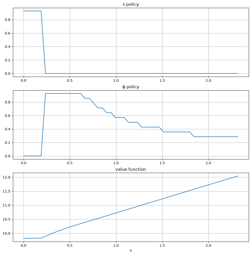
The horizontal axis is the state \(x\), while the vertical axis gives \(s(x)\) and \(\phi(x)\).
Overall, the policies match well with our predictions from above
Worker switches from one investment strategy to the other depending on relative return.
For low values of \(x\), the best option is to search for a new job.
Once \(x\) is larger, worker does better by investing in human capital specific to the current position.
56.5. Exercises#
Exercise 56.1
Let’s look at the dynamics for the state process \(\{x_t\}\) associated with these policies.
The dynamics are given by (56.1) when \(\phi_t\) and \(s_t\) are chosen according to the optimal policies, and \(\mathbb{P}\{b_{t+1} = 1\} = \pi(s_t)\).
Since the dynamics are random, analysis is a bit subtle.
One way to do it is to plot, for each \(x\) in a relatively fine grid
called plot_grid, a
large number \(K\) of realizations of \(x_{t+1}\) given \(x_t =
x\).
Plot this with one dot for each realization, in the form of a 45 degree diagram, setting
jv = create_jv_worker(grid_size=25, mc_size=50)
plot_grid_max, plot_grid_size = 1.2, 100
plot_grid = jnp.linspace(0, plot_grid_max, plot_grid_size)
fig, ax = plt.subplots()
ax.set_xlim(0, plot_grid_max)
ax.set_ylim(0, plot_grid_max)
By examining the plot, argue that under the optimal policies, the state \(x_t\) will converge to a constant value \(\bar x\) close to unity.
Argue that at the steady state, \(s_t \approx 0\) and \(\phi_t \approx 0.6\).
Solution
Here’s code to produce the 45 degree diagram.
Note that we draw all of the realizations at once, rather than looping over states and draws.
jv = create_jv_worker(grid_size=25, mc_size=50)
v_star, _, _ = solve_model(jv)
s_policy, ϕ_policy = get_greedy(v_star, jv)

# Turn the policy function arrays into actual functions
s = lambda y: jnp.interp(y, jv.x_grid, s_policy)
ϕ = lambda y: jnp.interp(y, jv.x_grid, ϕ_policy)

plot_grid_max, plot_grid_size = 1.2, 100
plot_grid = jnp.linspace(0, plot_grid_max, plot_grid_size)


@jax.jit
def simulate_next(key, plot_grid):
    """
    Draw realizations of next period capital for every x in plot_grid,
    following the law of motion for x_{t+1} given above.  Returns an array of shape (len(plot_grid), mc_size).
    """
    K = len(jv.f_rvs)
    gxϕ = g(jv, plot_grid, ϕ(plot_grid))[:, jnp.newaxis]   # Shape (n, 1)
    u = jv.f_rvs[jnp.newaxis, :]                           # Shape (1, K)

    # An offer arrives with probability π(s(x)), independently across draws
    b = jr.uniform(key, (len(plot_grid), K)) < π(s(plot_grid))[:, jnp.newaxis]

    return jnp.where(b, jnp.maximum(gxϕ, u), gxϕ)


x_next = simulate_next(jr.key(1234), plot_grid)

fig, ax = plt.subplots(figsize=(8, 8))
ticks = (0.25, 0.5, 0.75, 1.0)
ax.set(xticks=ticks, yticks=ticks,
       xlim=(0, plot_grid_max),
       ylim=(0, plot_grid_max),
       xlabel='$x_t$', ylabel='$x_{t+1}$')

ax.plot(plot_grid, plot_grid, 'k--', alpha=0.6)  # 45 degree line
ax.plot(jnp.repeat(plot_grid, x_next.shape[1]), x_next.ravel(),
        'go', alpha=0.25)

plt.show()
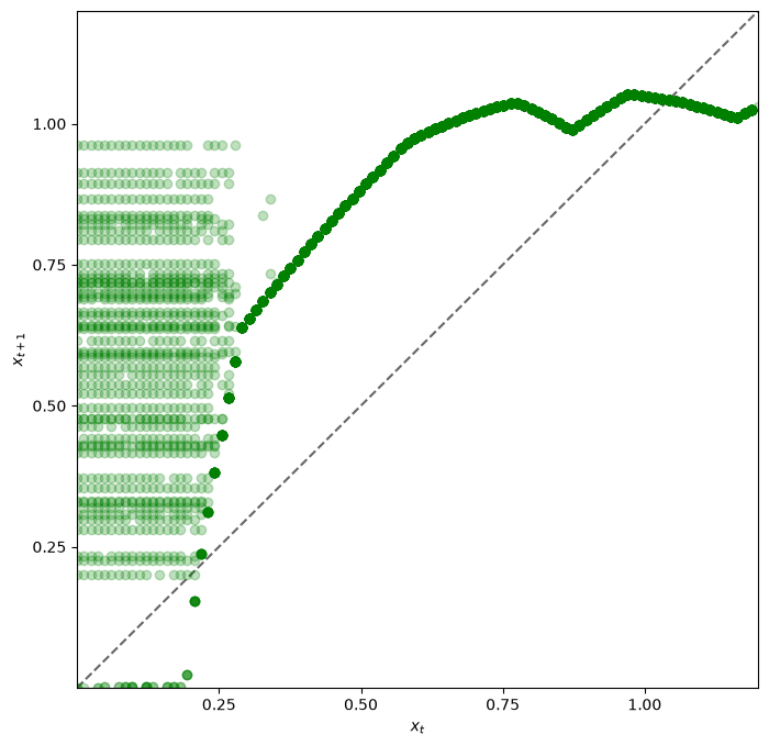
Looking at the dynamics, we can see that
If \(x_t\) is below about 0.2 the dynamics are random, but \(x_{t+1} > x_t\) is very likely.
As \(x_t\) increases the dynamics become deterministic, and \(x_t\) converges to a steady state value close to 1.
Referring back to the figure here we see that \(x_t \approx 1\) means that \(s_t = s(x_t) \approx 0\) and \(\phi_t = \phi(x_t) \approx 0.6\).
Exercise 56.2
In Exercise 56.1, we found that \(s_t\) converges to zero and \(\phi_t\) converges to about 0.6.
Since these results were calculated at a value of \(\beta\) close to one, let’s compare them to the best choice for an infinitely patient worker.
Intuitively, an infinitely patient worker would like to maximize steady state wages, which are a function of steady state capital.
You can take it as given—it’s certainly true—that the infinitely patient worker does not search in the long run (i.e., \(s_t = 0\) for large \(t\)).
Thus, given \(\phi\), steady state capital is the positive fixed point \(x^*(\phi)\) of the map \(x \mapsto g(x, \phi)\).
Steady state wages can be written as \(w^*(\phi) = x^*(\phi) (1 - \phi)\).
Graph \(w^*(\phi)\) with respect to \(\phi\), and examine the best choice of \(\phi\).
Can you give a rough interpretation for the value that you see?
Solution
The figure can be produced as follows
jv = create_jv_worker()

def xbar(ϕ):
    return (jv.A * ϕ**jv.α)**(1 / (1 - jv.α))

ϕ_grid = jnp.linspace(0, 1, 100)

fig, ax = plt.subplots(figsize=(9, 7))
ax.set(xlabel=r'$\phi$')
ax.plot(ϕ_grid, xbar(ϕ_grid) * (1 - ϕ_grid), label=r'$w^*(\phi)$')
ax.legend()

plt.show()
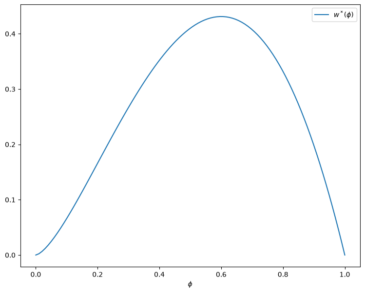
Observe that the maximizer is around 0.6.
This is similar to the long-run value for \(\phi\) obtained in Exercise 56.1.
Hence the behavior of the infinitely patent worker is similar to that of the worker with \(\beta = 0.96\).
This seems reasonable and helps us confirm that our dynamic programming solutions are probably correct.