55. Job Search VI: Modeling Career Choice #

GPU

This lecture was built using a machine with access to a GPU — although it will also run without one.

Google Colab has a free tier with GPUs that you can access as follows:

Click on the “play” icon top right
Select Colab
Set the runtime environment to include a GPU

In addition to what’s in Anaconda, this lecture will need the following libraries:

!pip install quantecon

55.1. Overview #

Next, we study a computational problem concerning career and job choices.

The model is originally due to Derek Neal [Neal, 1999].

This exposition draws on the presentation in [Ljungqvist and Sargent, 2018], section 6.5.

We begin with some imports:

from typing import NamedTuple

import matplotlib.pyplot as plt
from matplotlib import cm
from mpl_toolkits.mplot3d.axes3d import Axes3D
import jax
import jax.numpy as jnp
import jax.random as jr
from quantecon.distributions import BetaBinomial

55.1.1. Model Features#

Career and job within career both chosen to maximize expected discounted wage flow.
Infinite horizon dynamic programming with two state variables.

55.2. Model #

In what follows we distinguish between a career and a job, where

a career is understood to be a general field encompassing many possible jobs, and
a job is understood to be a position with a particular firm

For workers, wages can be decomposed into the contribution of job and career

\(w_t = \theta_t + \epsilon_t\), where
- \(\theta_t\) is the contribution of career at time \(t\)
- \(\epsilon_t\) is the contribution of the job at time \(t\)

At the start of time \(t\), a worker has the following options

retain a current (career, job) pair \((\theta_t, \epsilon_t)\) — referred to hereafter as “stay put”
retain a current career \(\theta_t\) but redraw a job \(\epsilon_t\) — referred to hereafter as “new job”
redraw both a career \(\theta_t\) and a job \(\epsilon_t\) — referred to hereafter as “new life”

Draws of \(\theta\) and \(\epsilon\) are independent of each other and past values, with

\(\theta_t \sim F\)
\(\epsilon_t \sim G\)

Notice that the worker does not have the option to retain a job but redraw a career — starting a new career always requires starting a new job.

A young worker aims to maximize the expected sum of discounted wages

(55.1)#\[\mathbb{E} \sum_{t=0}^{\infty} \beta^t w_t\]

subject to the choice restrictions specified above.

Let \(v(\theta, \epsilon)\) denote the value function, which is the maximum of (55.1) overall feasible (career, job) policies, given the initial state \((\theta, \epsilon)\).

The value function obeys

\[ v(\theta, \epsilon) = \max\{I, II, III\} \]

where

(55.2)#\[\begin{split}\begin{aligned} & I = \theta + \epsilon + \beta v(\theta, \epsilon) \\ & II = \theta + \int \epsilon' G(d \epsilon') + \beta \int v(\theta, \epsilon') G(d \epsilon') \nonumber \\ & III = \int \theta' F(d \theta') + \int \epsilon' G(d \epsilon') + \beta \int \int v(\theta', \epsilon') G(d \epsilon') F(d \theta') \nonumber \end{aligned}\end{split}\]

Evidently \(I\), \(II\) and \(III\) correspond to “stay put”, “new job” and “new life”, respectively.

55.2.1. Parameterization#

As in [Ljungqvist and Sargent, 2018], section 6.5, we will focus on a discrete version of the model, parameterized as follows:

both \(\theta\) and \(\epsilon\) take values in the set jnp.linspace(0, B, grid_size) — an even grid of points between \(0\) and \(B\) inclusive
grid_size = 50
B = 5
β = 0.95

The distributions \(F\) and \(G\) are discrete distributions generating draws from the grid points jnp.linspace(0, B, grid_size).

A very useful family of discrete distributions is the Beta-binomial family, with probability mass function

\[ p(k \,|\, n, a, b) = {n \choose k} \frac{B(k + a, n - k + b)}{B(a, b)}, \qquad k = 0, \ldots, n \]

Interpretation:

draw \(q\) from a Beta distribution with shape parameters \((a, b)\)
run \(n\) independent binary trials, each with success probability \(q\)
\(p(k \,|\, n, a, b)\) is the probability of \(k\) successes in these \(n\) trials

Nice properties:

very flexible class of distributions, including uniform, symmetric unimodal, etc.
only three parameters

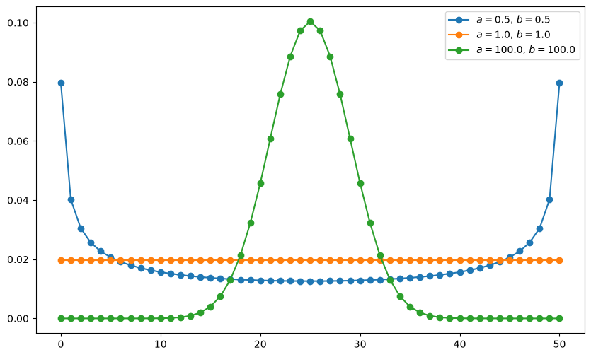
Here’s a figure showing the effect on the pmf of different shape parameters when \(n=50\).

n = 50
a_vals = [0.5, 1, 100]
b_vals = [0.5, 1, 100]

fig, ax = plt.subplots(figsize=(10, 6))
for a, b in zip(a_vals, b_vals):
    ab_label = f'$a = {a:.1f}$, $b = {b:.1f}$'
    ax.plot(range(n + 1), BetaBinomial(n, a, b).pdf(), '-o', label=ab_label)
ax.legend()
plt.show()

_images/295fb1143db39a5c7ac7e6409d756f6eabfc2049481b140766daa087a9e541ec.png

55.3. Implementation #

We store the model primitives in a NamedTuple, built by a factory function.

class CareerWorkerProblem(NamedTuple):
    β: float                 # Discount factor
    θ: jnp.ndarray           # Set of θ values (career)
    ϵ: jnp.ndarray           # Set of ϵ values (job)
    F_probs: jnp.ndarray     # Distribution over new career draws
    G_probs: jnp.ndarray     # Distribution over new job draws
    F_mean: float            # Mean of F
    G_mean: float            # Mean of G


def create_career_worker_problem(B=5.0,          # Upper bound
                                 β=0.95,         # Discount factor
                                 grid_size=50,   # Grid size
                                 F_a=1,
                                 F_b=1,
                                 G_a=1,
                                 G_b=1):
    "Create an instance of the career choice model."
    θ = jnp.linspace(0, B, grid_size)
    ϵ = jnp.linspace(0, B, grid_size)

    F_probs = jnp.array(BetaBinomial(grid_size - 1, F_a, F_b).pdf())
    G_probs = jnp.array(BetaBinomial(grid_size - 1, G_a, G_b).pdf())

    return CareerWorkerProblem(β=β, θ=θ, ϵ=ϵ,
                               F_probs=F_probs, G_probs=G_probs,
                               F_mean=θ @ F_probs, G_mean=ϵ @ G_probs)

The Bellman operator is \(Tv(\theta, \epsilon) = \max\{I, II, III\}\), where \(I\), \(II\) and \(III\) are as given in (55.2).

We start by writing those three values for a single state \((\theta_i, \epsilon_j)\), so that the code sits close to the equation.

def _B(v, cw, i, j):
    """
    The values of the three options available at state (θ_i, ϵ_j), in the
    order they appear in the Bellman equation.
    """
    stay_put = cw.θ[i] + cw.ϵ[j] + cw.β * v[i, j]                        # I
    new_job = cw.θ[i] + cw.G_mean + cw.β * v[i, :] @ cw.G_probs          # II
    new_life = cw.G_mean + cw.F_mean + cw.β * cw.F_probs @ v @ cw.G_probs # III
    return jnp.array([stay_put, new_job, new_life])

Now we evaluate _B at every state.

Rather than write two nested loops over \(i\) and \(j\), we apply jax.vmap twice.

In in_axes, a 0 marks the argument being mapped over, while None holds an argument fixed.

# The argument order of _B is  (v,    cw,   i,    j)
_B_j  = jax.vmap(_B,   in_axes=(None, None, None, 0))   # over j
_B_ij = jax.vmap(_B_j, in_axes=(None, None, 0,    None))  # then over i


@jax.jit
def B(v, cw):
    "Value of each option at each state; shape (grid_size, grid_size, 3)."
    n = len(cw.θ)
    return _B_ij(v, cw, jnp.arange(n), jnp.arange(n))

The Bellman operator and the greedy policy are now the maximum and the maximizer of the same array.

@jax.jit
def T(v, cw):
    "The Bellman operator."
    return jnp.max(B(v, cw), axis=-1)


@jax.jit
def get_greedy(v, cw):
    "The v-greedy policy, coded as 1 = stay put, 2 = new job, 3 = new life."
    return jnp.argmax(B(v, cw), axis=-1) + 1

Lastly, solve_model iterates the Bellman operator to find the fixed point.

We use jax.lax.while_loop so that the whole iteration compiles into a single operation, and bound the number of steps so the loop always terminates.

@jax.jit
def solve_model(cw, tol=1e-4, max_iter=1_000):
    """
    Solve the model by value function iteration.

    Returns the value function, the number of iterations taken and the final
    error, so that the caller can check convergence.
    """
    def condition(loop_state):
        i, v, error = loop_state
        return (error > tol) & (i < max_iter)

    def update(loop_state):
        i, v, error = loop_state
        v_new = T(v, cw)
        return i + 1, v_new, jnp.max(jnp.abs(v_new - v))

    n = len(cw.θ)
    v_init = jnp.full((n, n), 100.0)
    i, v, error = jax.lax.while_loop(condition, update, (0, v_init, tol + 1))
    return v, i, error

Note

The grid here is small, and this model would also run perfectly well in NumPy.

We use JAX because the code is almost as readable as the NumPy equivalent while scaling far better — to finer grids, or to richer versions of the model with more state variables, where the same code will make full use of a GPU.

The gain is already visible in Exercise 55.2, where we simulate 25,000 independent careers at once.

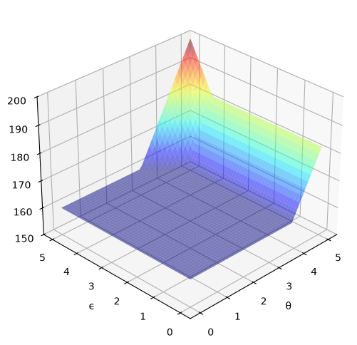
Here’s the solution to the model – an approximate value function

cw = create_career_worker_problem()
v_star, num_iter, error = solve_model(cw)
greedy_star = get_greedy(v_star, cw)

print(f"Converged in {num_iter} iterations with error {error:.2e}.")

fig = plt.figure(figsize=(8, 6))
ax = fig.add_subplot(111, projection='3d')
tg, eg = jnp.meshgrid(cw.θ, cw.ϵ)
ax.plot_surface(tg,
                eg,
                v_star.T,
                cmap=cm.jet,
                alpha=0.5,
                linewidth=0.25)
ax.set(xlabel='θ', ylabel='ϵ', zlim=(150, 200))
ax.view_init(ax.elev, 225)
plt.show()

Converged in 213 iterations with error 9.16e-05.

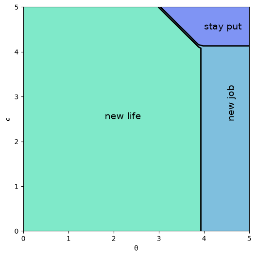
_images/cf2d639de64f4128b6afe6c4470e68e09511799b76732a2752c01735f67a3329.png

And here is the optimal policy

fig, ax = plt.subplots(figsize=(6, 6))
tg, eg = jnp.meshgrid(cw.θ, cw.ϵ)
lvls = (0.5, 1.5, 2.5, 3.5)
ax.contourf(tg, eg, greedy_star.T, levels=lvls, cmap=cm.winter, alpha=0.5)
ax.contour(tg, eg, greedy_star.T, colors='k', levels=lvls, linewidths=2)
ax.set(xlabel='θ', ylabel='ϵ')
ax.text(1.8, 2.5, 'new life', fontsize=14)
ax.text(4.5, 2.5, 'new job', fontsize=14, rotation='vertical')
ax.text(4.0, 4.5, 'stay put', fontsize=14)
plt.show()

_images/5a5be44866085eda8cb52a641319fd9f5efab89e3067fe34486a6846d772bdc9.png

Interpretation:

If both job and career are poor or mediocre, the worker will experiment with a new job and new career.
If career is sufficiently good, the worker will hold it and experiment with new jobs until a sufficiently good one is found.
If both job and career are good, the worker will stay put.

Notice that the worker will always hold on to a sufficiently good career, but not necessarily hold on to even the best paying job.

The reason is that high lifetime wages require both a good job and a good career, but the worker cannot change careers without changing jobs.

Sometimes a good job must be sacrificed in order to change to a better career.

55.4. Exercises #

Exercise 55.1

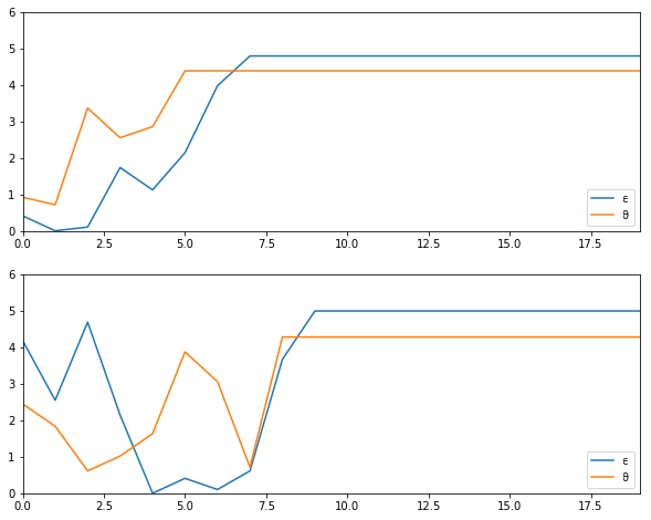
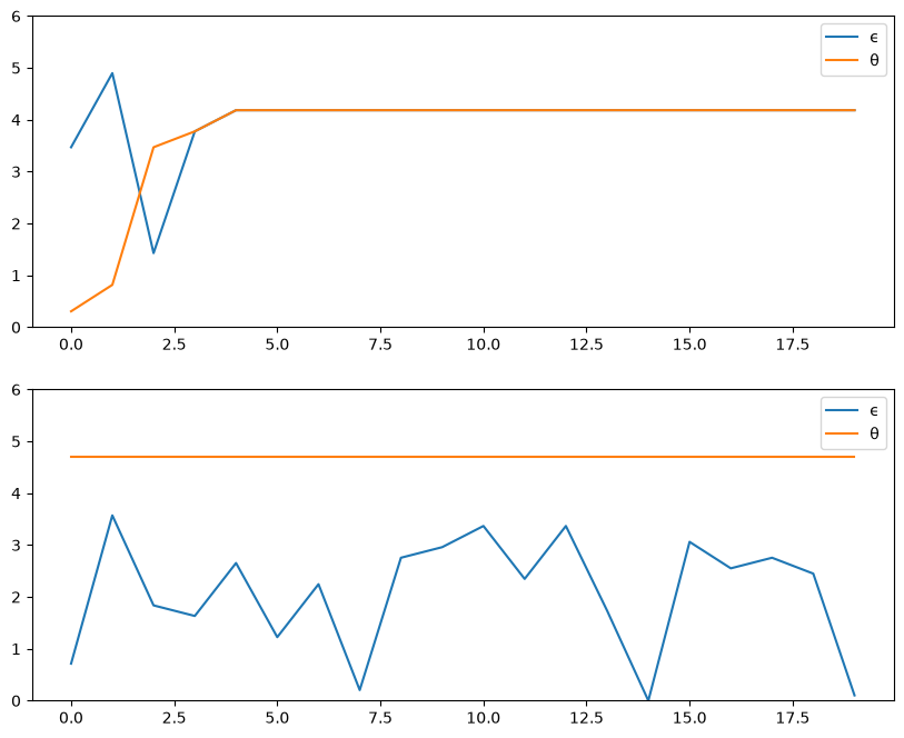
Using the default parameterization in the function create_career_worker_problem, generate and plot typical sample paths for \(\theta\) and \(\epsilon\) when the worker follows the optimal policy.

In particular, modulo randomness, reproduce the following figure (where the horizontal axis represents time)

Hint

To draw from \(F\) and \(G\), invert their cdfs with jnp.searchsorted.

Solution

Simulate job/career paths.

In reading the code, recall that greedy_star[i, j] = policy at \((\theta_i, \epsilon_j)\) = either 1, 2 or 3; meaning ‘stay put’, ‘new job’ and ‘new life’.

def draw(key, cdf):
    "Draw an index from the distribution with the given cdf."
    return jnp.searchsorted(cdf, jr.uniform(key), side="right")


def simulate_path(cw, greedy_star, key, t=20):
    "Simulate a career/job path of length t under the greedy policy."
    F_cdf, G_cdf = jnp.cumsum(cw.F_probs), jnp.cumsum(cw.G_probs)

    def update(state, key):
        i, j = state
        action = greedy_star[i, j]
        key_F, key_G = jr.split(key)
        # Career changes only under 'new life'; the job changes unless we stay put
        i_new = jnp.where(action == 3, draw(key_F, F_cdf), i)
        j_new = jnp.where(action == 1, j, draw(key_G, G_cdf))
        return (i_new, j_new), (i_new, j_new)

    _, (i_path, j_path) = jax.lax.scan(update, (0, 0), jr.split(key, t))
    return cw.θ[i_path], cw.ϵ[j_path]


cw = create_career_worker_problem()
v_star, _, _ = solve_model(cw)
greedy_star = get_greedy(v_star, cw)

key = jr.key(42)
fig, axes = plt.subplots(2, 1, figsize=(10, 8))

for ax in axes:
    key, subkey = jr.split(key)
    θ_path, ϵ_path = simulate_path(cw, greedy_star, subkey)
    ax.plot(ϵ_path, label='ϵ')
    ax.plot(θ_path, label='θ')
    ax.set_ylim(0, 6)
    ax.legend()

plt.show()

_images/7227cf54e0c2e0491990af22ca267dec7ef3236a79bab00846250d64064adfb7.png

Exercise 55.2

Let’s now consider how long it takes for the worker to settle down to a permanent job, given a starting point of \((\theta, \epsilon) = (0, 0)\).

In other words, we want to study the distribution of the random variable

\[ T^* := \text{the first point in time from which the worker's job no longer changes} \]

Evidently, the worker’s job becomes permanent if and only if \((\theta_t, \epsilon_t)\) enters the “stay put” region of \((\theta, \epsilon)\) space.

Letting \(S\) denote this region, \(T^*\) can be expressed as the first passage time to \(S\) under the optimal policy:

\[ T^* := \inf\{t \geq 0 \,|\, (\theta_t, \epsilon_t) \in S\} \]

Collect 25,000 draws of this random variable and compute the median (which should be about 7).

Repeat the exercise with \(\beta=0.99\) and interpret the change.

Solution

The median for the original parameterization can be computed as follows.

Each simulation is an independent sequential search, so we write one with jax.lax.while_loop and then run 25,000 of them at once with jax.vmap.

def passage_time(cw, greedy_star, key, max_t=1_000):
    "Time until the worker first chooses to stay put."
    F_cdf, G_cdf = jnp.cumsum(cw.F_probs), jnp.cumsum(cw.G_probs)

    def condition(state):
        i, j, t, key = state
        return (greedy_star[i, j] != 1) & (t < max_t)

    def update(state):
        i, j, t, key = state
        action = greedy_star[i, j]
        key, key_F, key_G = jr.split(key, 3)
        i_new = jnp.where(action == 3, draw(key_F, F_cdf), i)
        j_new = jnp.where(action == 1, j, draw(key_G, G_cdf))
        return i_new, j_new, t + 1, key

    _, _, t, _ = jax.lax.while_loop(condition, update, (0, 0, 0, key))
    return t


@jax.jit
def median_passage_time(cw, greedy_star, key, M=25_000):
    "Median time to settle down, over M independent simulations."
    keys = jr.split(key, M)
    times = jax.vmap(passage_time, in_axes=(None, None, 0))(cw, greedy_star, keys)
    return jnp.median(times)


median_passage_time(cw, greedy_star, jr.key(42))

Array(7., dtype=float32)

To compute the median with \(\beta=0.99\) instead of the default value \(\beta=0.95\), we create a new instance and solve it again.

cw_patient = create_career_worker_problem(β=0.99)
v_patient, _, _ = solve_model(cw_patient)
greedy_patient = get_greedy(v_patient, cw_patient)

median_passage_time(cw_patient, greedy_patient, jr.key(42))

Array(14., dtype=float32)

The medians are subject to randomness but should be about 7 and 14 respectively.

Not surprisingly, more patient workers will wait longer to settle down to their final job.

Exercise 55.3

Set the parameterization to G_a = G_b = 100 and generate a new optimal policy figure – interpret.

Solution

Here is one solution

cw = create_career_worker_problem(G_a=100, G_b=100)
v_star, _, _ = solve_model(cw)
greedy_star = get_greedy(v_star, cw)

fig, ax = plt.subplots(figsize=(6, 6))
tg, eg = jnp.meshgrid(cw.θ, cw.ϵ)
lvls = (0.5, 1.5, 2.5, 3.5)
ax.contourf(tg, eg, greedy_star.T, levels=lvls, cmap=cm.winter, alpha=0.5)
ax.contour(tg, eg, greedy_star.T, colors='k', levels=lvls, linewidths=2)
ax.set(xlabel='θ', ylabel='ϵ')
ax.text(1.8, 2.5, 'new life', fontsize=14)
ax.text(4.5, 1.5, 'new job', fontsize=14, rotation='vertical')
ax.text(4.0, 4.5, 'stay put', fontsize=14)
plt.show()

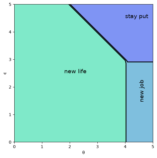
_images/7bb8c646c687144268510da4faa4812ecbde1c037f491d97e1b4e5c2df38767a.png

In the new figure, you see that the region for which the worker stays put has grown because the distribution for \(\epsilon\) has become more concentrated around the mean, making high-paying jobs less realistic.

55. Job Search VI: Modeling Career Choice#

55.1. Overview#

55.1.1. Model Features#

55.2. Model#

55.2.1. Parameterization#

55.3. Implementation#

55.4. Exercises#

55. Job Search VI: Modeling Career Choice #

55.1. Overview #

55.2. Model #

55.3. Implementation #

55.4. Exercises #