25. Mean of a Likelihood Ratio Process#
25.1. Overview#
In Likelihood Ratio Processes we described a peculiar property of a likelihood ratio process, namely, that its mean equals one for all \(t \geq 0\) despite its converging to zero almost surely.
While it is easy to verify that peculiar property analytically (i.e., in population), it is challenging to use a computer simulation to verify it via an application of a law of large numbers that entails studying sample averages of repeated simulations.
To confront this challenge, this lecture puts importance sampling to work to accelerate convergence of sample averages to population means.
We use importance sampling to estimate the mean of a cumulative likelihood ratio \(L\left(\omega^t\right) = \prod_{i=1}^t \ell \left(\omega_i\right)\).
We start by importing some Python packages.
import jax
import jax.numpy as jnp
import matplotlib.pyplot as plt
from jax.scipy.special import gammaln
from typing import NamedTuple
from functools import partial

# Set JAX to use 64-bit floats
jax.config.update("jax_enable_x64", True)
Matplotlib is building the font cache; this may take a moment.
25.2. Mathematical expectation of likelihood ratio#
In Likelihood Ratio Processes, we studied a likelihood ratio \(\ell \left(\omega_t\right)\)
where \(f\) and \(g\) are densities for Beta distributions with parameters \(F_a\), \(F_b\), \(G_a\), \(G_b\).
Assume that an i.i.d. random variable \(\omega_t \in \Omega\) is generated by \(g\).
The cumulative likelihood ratio \(L \left(\omega^t\right)\) is
Our goal is to approximate the mathematical expectation \(E \left[ L\left(\omega^t\right) \right]\) well.
In Likelihood Ratio Processes, we showed that \(E \left[ L\left(\omega^t\right) \right]\) equals \(1\) for all \(t\).
We want to check out how well this holds if we replace \(E\) with sample averages from simulations.
This turns out to be easier said than done because for Beta distributions assumed above, \(L\left(\omega^t\right)\) has a very skewed distribution with a very long tail as \(t \rightarrow \infty\).
This property makes it difficult efficiently and accurately to estimate the mean by standard Monte Carlo simulation methods.
In this lecture we explore how a standard Monte Carlo method fails.
We also show how importance sampling provides a more computationally efficient way to approximate the mean of the cumulative likelihood ratio.
We first take a look at the density functions f and g .
# Parameters for the model
class ImpSampleParams(NamedTuple):
    F_a: float = 1.0    # Beta parameters for f
    F_b: float = 1.0
    G_a: float = 3.0    # Beta parameters for g
    G_b: float = 1.2

params = ImpSampleParams()

@jax.jit
def beta_pdf(w, a, b):
    """Beta probability density function."""
    log_beta_const = (gammaln(a) + gammaln(b) -
                      gammaln(a + b))
    log_pdf = ((a - 1) * jnp.log(w) + (b - 1) *
               jnp.log(1 - w) - log_beta_const)
    return jnp.exp(log_pdf)

@jax.jit
def f(w, params=params):
    return beta_pdf(w, params.F_a, params.F_b)

@jax.jit
def g(w, params=params):
    return beta_pdf(w, params.G_a, params.G_b)
w_range = jnp.linspace(1e-2, 1-1e-5, 1000)

plt.plot(w_range, g(w_range), lw=2, label='g')
plt.plot(w_range, f(w_range), lw=2, label='f')
plt.xlabel(r'$\omega$')
plt.legend()
plt.show()
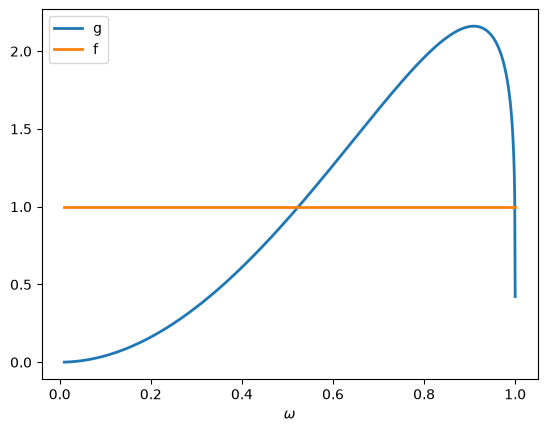
Fig. 25.1 Beta density functions \(f\) and \(g\)#
The likelihood ratio is l(w)=f(w)/g(w).
@jax.jit
def l(w):
    return f(w) / g(w)
plt.plot(w_range, l(w_range), lw=2)
plt.xlabel(r'$\omega$')
plt.show()
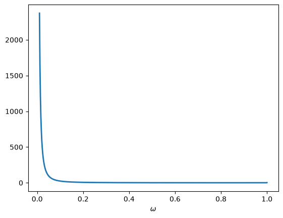
Fig. 25.2 Likelihood ratio \(\ell(\omega)\)#
The above plots shows that as \(\omega \rightarrow 0\), \(f \left(\omega\right)\) is unchanged and \(g \left(\omega\right) \rightarrow 0\), so the likelihood ratio approaches infinity.
A Monte Carlo approximation of \(\hat{E} \left[L\left(\omega^t\right)\right] = \hat{E} \left[\prod_{i=1}^t \ell \left(\omega_i\right)\right]\) would repeatedly draw \(\omega\) from \(g\), calculate the likelihood ratio \( \ell(\omega) = \frac{f(\omega)}{g(\omega)}\) for each draw, then average these over all draws.
Because \(g(\omega) \rightarrow 0\) as \(\omega \rightarrow 0\), such a simulation procedure undersamples a part of the sample space \([0,1]\) that it is important to visit often in order to do a good job of approximating the mathematical expectation of the likelihood ratio \(\ell(\omega)\).
We illustrate this numerically below.
25.3. Importance sampling#
We circumvent the issue by using a change of distribution called importance sampling.
Instead of drawing from \(g\) to generate data during the simulation, we use an alternative distribution \(h\) to generate draws of \(\omega\).
The idea is to design \(h\) so that it oversamples the region of \(\Omega\) where \(\ell \left(\omega_t\right)\) has large values but low density under \(g\).
After we construct a sample in this way, we must then weight each realization by the likelihood ratio of \(g\) and \(h\) when we compute the empirical mean of the likelihood ratio.
By doing this, we properly account for the fact that we are using \(h\) and not \(g\) to simulate data.
To illustrate, suppose were interested in \({E}\left[\ell\left(\omega\right)\right]\).
We could simply compute:
where \(\omega_i^g\) indicates that \(\omega_i\) is drawn from \(g\).
But using our insight from importance sampling, we could instead calculate the object:
where \(w_i\) is now drawn from importance distribution \(h\).
Notice that the above two are exactly the same population objects:
25.4. Selecting a sampling distribution#
Since we must use an \(h\) that has larger mass in parts of the distribution to which \(g\) puts low mass, we use \(h=Beta(0.5, 0.5)\) as our importance distribution.
The plots compare \(g\) and \(h\).
g_a, g_b = params.G_a, params.G_b
h_a, h_b = 0.5, 0.5
w_range = jnp.linspace(1e-5, 1-1e-5, 1000)

plt.plot(w_range, g(w_range),
         lw=2, label=f'g=Beta({g_a}, {g_b})')
plt.plot(w_range, beta_pdf(w_range, 0.5, 0.5),
         lw=2, label=f'h=Beta({h_a}, {h_b})')
plt.legend()
plt.ylim([0., 3.])
plt.show()
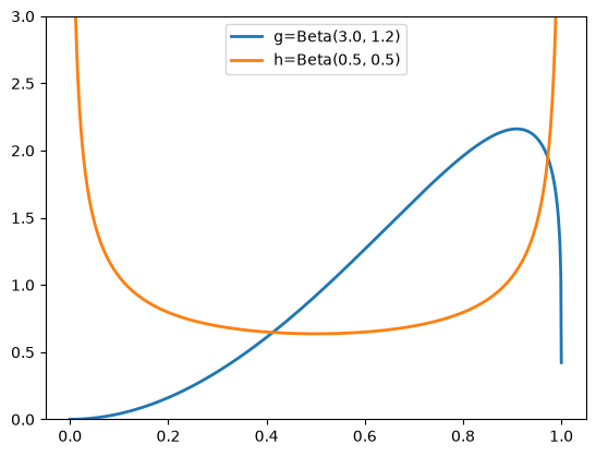
Fig. 25.3 Data and importance sampling distributions#
25.5. Approximating a cumulative likelihood ratio#
We now study how to use importance sampling to approximate \({E} \left[L(\omega^t)\right] = \left[\prod_{i=1}^T \ell \left(\omega_i\right)\right]\).
As above, our plan is to draw sequences \(\omega^t\) from \(q\) and then re-weight the likelihood ratio appropriately:
where the last equality uses \(\omega_{i,t}^h\) drawn from the importance distribution \(q\).
Here \(\frac{p\left(\omega_{i,t}^q\right)}{q\left(\omega_{i,t}^q\right)}\) is the weight we assign to each data point \(\omega_{i,t}^q\).
Below we prepare a Python function for computing the importance sampling estimates given any beta distributions \(p\), \(q\).
@jax.jit
def estimate_single_path(key, p_a, p_b, q_a, q_b, T):
    """
    Estimation for a single sample path.
    """

    def loop_body(i, carry):
        L, weight, key_state = carry
        key_state, subkey = jax.random.split(key_state)
        w = jax.random.beta(subkey, q_a, q_b)

        # Compute likelihood ratio using f/g functions
        likelihood_ratio = f(w) / g(w)
        L = L * likelihood_ratio

        # Importance sampling weight with beta_pdf
        p_w = beta_pdf(w, p_a, p_b)
        q_w = beta_pdf(w, q_a, q_b)
        weight = weight * (p_w / q_w)

        return (L, weight, key_state)

    # Use fori_loop for dynamic T values
    final_L, final_weight, _ = jax.lax.fori_loop(
        0, T, loop_body, (1.0, 1.0, key)
    )
    return final_L * final_weight

@partial(jax.jit, static_argnames=['N'])
def estimate(key, p_a, p_b, q_a, q_b, T=1, N=10000):
    """Estimation of a batch of sample paths."""
    keys = jax.random.split(key, N)

    # Use vmap for vectorized computation
    estimates = jax.vmap(
        estimate_single_path,
        in_axes=(0, *[None]*5)
    )(keys, p_a, p_b, q_a, q_b, T)

    return jnp.mean(estimates)
Consider the case when \(T=1\), which amounts to approximating \(E_0\left[\ell\left(\omega\right)\right]\)
For the standard Monte Carlo estimate, we can set \(p=g\) and \(q=g\).
estimate(jax.random.key(0), g_a, g_b, g_a, g_b,
         T=1, N=10000)
Array(0.98300826, dtype=float64)
For our importance sampling estimate, we set \(q = h\).
estimate(jax.random.key(1), g_a, g_b, h_a, h_b,
         T=1, N=10000)
Array(1.00722995, dtype=float64)
Evidently, even at \(T=1\), our importance sampling estimate is closer to \(1\) than is the Monte Carlo estimate.
Bigger differences arise when computing expectations over longer sequences, \(E_0\left[L\left(\omega^t\right)\right]\).
Setting \(T=10\), we find that the Monte Carlo method severely underestimates the mean while importance sampling still produces an estimate close to its theoretical value of unity.
estimate(jax.random.key(2), g_a, g_b, g_a, g_b,
         T=10, N=10000)
Array(0.60388316, dtype=float64)
estimate(jax.random.key(3), g_a, g_b, h_a, h_b,
         T=10, N=10000)
Array(0.99185478, dtype=float64)
The Monte Carlo method underestimates because the likelihood ratio \(L(\omega^T) = \prod_{t=1}^T \frac{f(\omega_t)}{g(\omega_t)}\) has a highly skewed distribution under \(g\).
Most samples from \(g\) produce small likelihood ratios, while the true mean requires occasional very large values that are rarely sampled.
In our case, since \(g(\omega) \to 0\) as \(\omega \to 0\) while \(f(\omega)\) remains constant, the Monte Carlo procedure undersamples precisely where the likelihood ratio \(\frac{f(\omega)}{g(\omega)}\) is largest.
As \(T\) increases, this problem worsens exponentially, making standard Monte Carlo increasingly unreliable.
Importance sampling with \(q = h\) fixes this by sampling more uniformly from regions important to both \(f\) and \(g\).
25.6. Distribution of sample mean#
We next study the bias and efficiency of the Monte Carlo and importance sampling approaches.
The code below produces distributions of estimates using both Monte Carlo and importance sampling methods.
@partial(jax.jit, static_argnames=['N_simu', 'N_samples'])
def simulate(key, p_a, p_b, q_a, q_b, N_simu, T=1,
             N_samples=10000):
    """Simulation for both Monte Carlo and importance sampling."""
    keys = jax.random.split(key, 2 * N_simu)
    keys_p = keys[:N_simu]
    keys_q = keys[N_simu:]

    def run_monte_carlo(key_batch):
        return estimate(key_batch, p_a, p_b, p_a, p_b, T,
                        N_samples)

    def run_importance_sampling(key_batch):
        return estimate(key_batch, p_a, p_b, q_a, q_b, T,
                        N_samples)

    μ_L_p = jax.vmap(run_monte_carlo)(keys_p)
    μ_L_q = jax.vmap(run_importance_sampling)(keys_q)

    return μ_L_p, μ_L_q
Again, we first consider estimating \({E} \left[\ell\left(\omega\right)\right]\) by setting T=1.
We simulate \(1000\) times for each method.
N_simu = 1000
μ_L_p, μ_L_q = simulate(jax.random.key(4), g_a, g_b,
                         h_a, h_b, N_simu)
# standard Monte Carlo (mean and std)
jnp.nanmean(μ_L_p), jnp.nanvar(μ_L_p)
(Array(0.99558545, dtype=float64), Array(0.00448641, dtype=float64))
# importance sampling (mean and std)
jnp.nanmean(μ_L_q), jnp.nanvar(μ_L_q)
(Array(1.00003504, dtype=float64), Array(2.29258849e-05, dtype=float64))
Although both methods tend to provide a mean estimate of \({E} \left[\ell\left(\omega\right)\right]\) close to \(1\), the importance sampling estimates have smaller variance.
Next, we present distributions of estimates for \(\hat{E} \left[L\left(\omega^t\right)\right]\), in cases for \(T=1, 5, 10, 20\).
def simulate_multiple_T(key, p_a, p_b, q_a, q_b, N_simu,
                        T_list, N_samples=10000):
    """Simulation for multiple T values."""
    n_T = len(T_list)
    keys = jax.random.split(key, n_T)

    results = []
    for i, T in enumerate(T_list):
        result = simulate(keys[i],
                          p_a, p_b, q_a, q_b, N_simu, T,
                          N_samples)
        results.append(result)

    # Stack results into arrays for consistency
    μ_L_p_all = jnp.stack([r[0] for r in results])
    μ_L_q_all = jnp.stack([r[1] for r in results])

    return μ_L_p_all, μ_L_q_all
T_values = [1, 5, 10, 20]

# Run all simulations at once
all_results = simulate_multiple_T(jax.random.key(5),
                                  g_a, g_b, h_a, h_b,
                                  N_simu, T_values,
                                  N_samples=10000)

# Extract results
μ_L_p_all, μ_L_q_all = all_results

fig, axs = plt.subplots(2, 2, figsize=(14, 10))
μ_range = jnp.linspace(0, 2, 100)

for i, t in enumerate(T_values):
    row = i // 2
    col = i % 2

    # Get results for this T value
    μ_L_p = μ_L_p_all[i]
    μ_L_q = μ_L_q_all[i]

    μ_hat_p = jnp.nanmean(μ_L_p)
    μ_hat_q = jnp.nanmean(μ_L_q)
    σ_hat_p = jnp.nanvar(μ_L_p)
    σ_hat_q = jnp.nanvar(μ_L_q)

    axs[row, col].set_xlabel('$μ_L$')
    axs[row, col].set_ylabel('frequency')
    axs[row, col].set_title(f'$T$={t}')
    n_p, bins_p, _ = axs[row, col].hist(
        μ_L_p, bins=μ_range,
        color='r', alpha=0.5, label='$g$ generating')
    n_q, bins_q, _ = axs[row, col].hist(
        μ_L_q, bins=μ_range,
        color='b', alpha=0.5, label='$h$ generating')
    axs[row, col].legend(loc=4)

    for n, bins, μ_hat, σ_hat in [[n_p, bins_p, μ_hat_p,
                                    σ_hat_p],
                                   [n_q, bins_q, μ_hat_q,
                                    σ_hat_q]]:
        idx = jnp.argmax(n)
        axs[row, col].text(
            bins[idx], n[idx],
            r'$\hat{μ}$=' + f'{μ_hat:.4g}' +
            r', $\hat{σ}=$' + f'{σ_hat:.4g}')

plt.show()
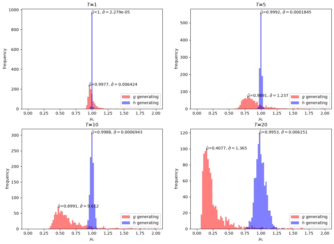
Fig. 25.4 Monte Carlo and importance sampling estimates#
The simulation exercises above show that the importance sampling estimates are unbiased under all \(T\) while the standard Monte Carlo estimates are biased downwards.
Evidently, the bias increases with increases in \(T\).
25.7. Choosing a sampling distribution#
Above, we arbitraily chose \(h = Beta(0.5,0.5)\) as the importance distribution.
Is there an optimal importance distribution?
In our particular case, since we know in advance that \(E_0 \left[ L\left(\omega^t\right) \right] = 1\), we can use that knowledge to our advantage.
Thus, suppose that we simply use \(h = f\).
When estimating the mean of the likelihood ratio (T=1), we get:
μ_L_p, μ_L_q = simulate(jax.random.key(6), g_a, g_b,
                         params.F_a, params.F_b, N_simu)
# importance sampling (mean and std)
jnp.nanmean(μ_L_q), jnp.nanvar(μ_L_q)
(Array(1., dtype=float64), Array(0., dtype=float64))
We could also use other distributions as our importance distribution.
Below we choose just a few and compare their sampling properties.
a_list = [0.5, 1., 2.]
b_list = [0.5, 1.2, 5.]
w_range = jnp.linspace(1e-5, 1-1e-5, 1000)

plt.plot(w_range, g(w_range),
         lw=2, label=f'g=Beta({g_a}, {g_b})')
plt.plot(w_range, beta_pdf(w_range, a_list[0], b_list[0]),
         lw=2, label=f'$h_1$=Beta({a_list[0]},{b_list[0]})')
plt.plot(w_range, beta_pdf(w_range, a_list[1], b_list[1]),
         lw=2, label=f'$h_2$=Beta({a_list[1]},{b_list[1]})')
plt.plot(w_range, beta_pdf(w_range, a_list[2], b_list[2]),
         lw=2, label=f'$h_3$=Beta({a_list[2]},{b_list[2]})')
plt.legend()
plt.ylim([0., 3.])
plt.show()
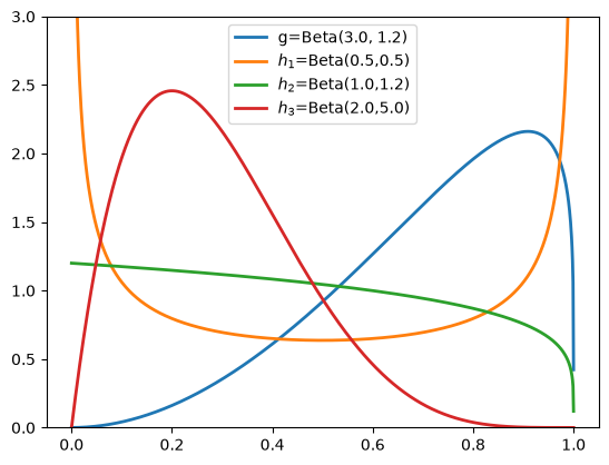
Fig. 25.5 Comparison of importance sampling distributions#
We consider two additional distributions.
As a reminder \(h_1\) is the original \(Beta(0.5,0.5)\) distribution that we used above.
\(h_2\) is the \(Beta(1,1.2)\) distribution.
Note how \(h_2\) has a similar shape to \(g\) at higher values of distribution but more mass at lower values.
Our hunch is that \(h_2\) should be a good importance sampling distribution.
\(h_3\) is the \(Beta(2,5)\) distribution.
Note how \(h_3\) has zero mass at values very close to 0 and at values close to 1.
Our hunch is that \(h_3\) will be a poor importance sampling distribution.
We first simulate a plot the distribution of estimates for \(\hat{E} \left[L\left(\omega^t\right)\right]\) using \(h_2\) as the importance sampling distribution.
h_a = a_list[1]
h_b = b_list[1]

T_values_h2 = [1, 20]
all_results_h2 = simulate_multiple_T(jax.random.key(7),
                                     g_a, g_b, h_a, h_b,
                                     N_simu, T_values_h2,
                                     N_samples=10000)
μ_L_p_all_h2, μ_L_q_all_h2 = all_results_h2

fig, axs = plt.subplots(1, 2, figsize=(14, 10))
μ_range = jnp.linspace(0, 2, 100)

for i, t in enumerate(T_values_h2):
    μ_L_p = μ_L_p_all_h2[i]
    μ_L_q = μ_L_q_all_h2[i]

    μ_hat_p = jnp.nanmean(μ_L_p)
    μ_hat_q = jnp.nanmean(μ_L_q)
    σ_hat_p = jnp.nanvar(μ_L_p)
    σ_hat_q = jnp.nanvar(μ_L_q)

    axs[i].set_xlabel('$μ_L$')
    axs[i].set_ylabel('frequency')
    axs[i].set_title(f'$T$={t}')
    n_p, bins_p, _ = axs[i].hist(
        μ_L_p, bins=μ_range,
        color='r', alpha=0.5, label='$g$ generating')
    n_q, bins_q, _ = axs[i].hist(
        μ_L_q, bins=μ_range,
        color='b', alpha=0.5, label='$h_2$ generating')
    axs[i].legend(loc=4)

    for n, bins, μ_hat, σ_hat in [[n_p, bins_p, μ_hat_p,
                                    σ_hat_p],
                                   [n_q, bins_q, μ_hat_q,
                                    σ_hat_q]]:
        idx = jnp.argmax(n)
        axs[i].text(
            bins[idx], n[idx],
            r'$\hat{μ}$=' + f'{μ_hat:.4g}' +
            r', $\hat{σ}=$' + f'{σ_hat:.4g}')

plt.show()
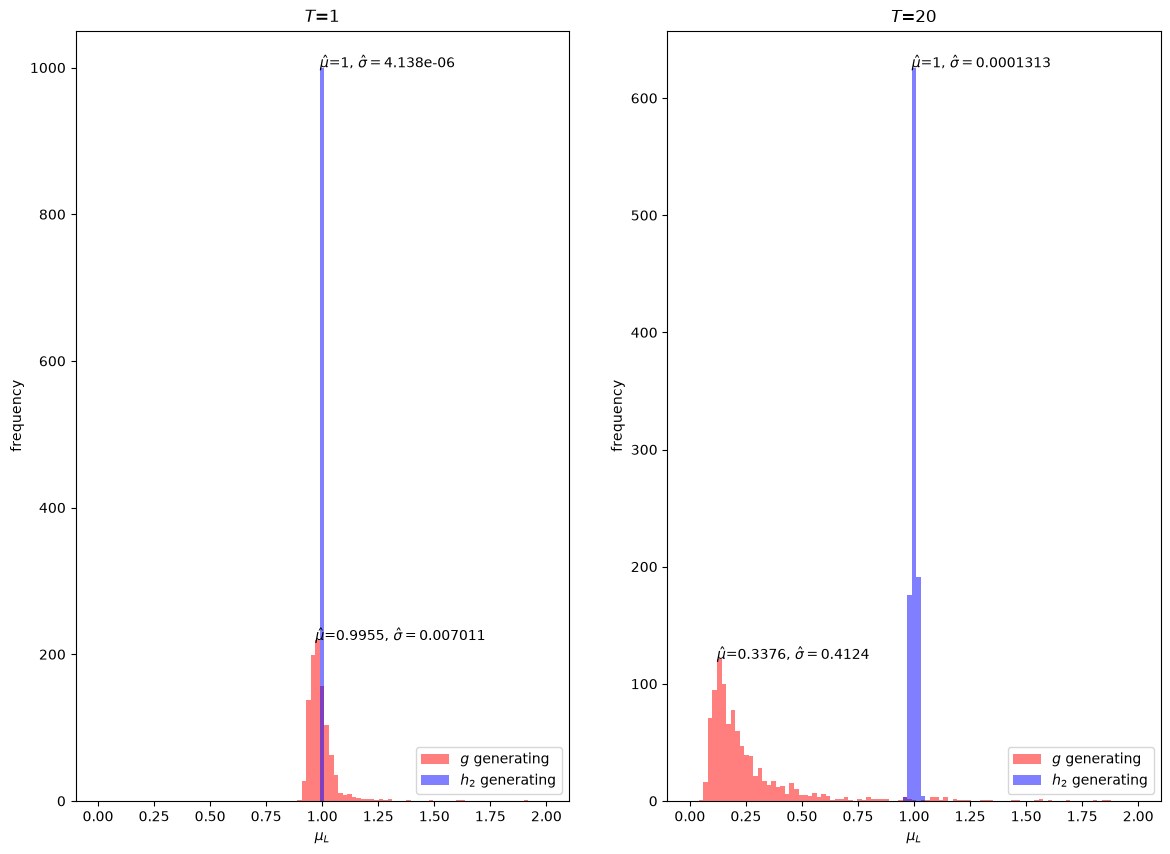
Fig. 25.6 Estimates using importance distribution \(h_2\)#
Our simulations suggest that indeed \(h_2\) is a quite good importance sampling distribution for our problem.
Even at \(T=20\), the mean is very close to \(1\) and the variance is small.
h_a = a_list[2]
h_b = b_list[2]

T_values_h3 = [1, 20]
all_results_h3 = simulate_multiple_T(jax.random.key(8),
                                     g_a, g_b, h_a, h_b,
                                     N_simu, T_values_h3,
                                     N_samples=10000)
μ_L_p_all_h3, μ_L_q_all_h3 = all_results_h3

fig, axs = plt.subplots(1, 2, figsize=(14, 10))
μ_range = jnp.linspace(0, 2, 100)

for i, t in enumerate(T_values_h3):
    μ_L_p = μ_L_p_all_h3[i]
    μ_L_q = μ_L_q_all_h3[i]
    μ_hat_p = jnp.nanmean(μ_L_p)
    μ_hat_q = jnp.nanmean(μ_L_q)
    σ_hat_p = jnp.nanvar(μ_L_p)
    σ_hat_q = jnp.nanvar(μ_L_q)

    axs[i].set_xlabel('$μ_L$')
    axs[i].set_ylabel('frequency')
    axs[i].set_title(f'$T$={t}')
    n_p, bins_p, _ = axs[i].hist(
        μ_L_p, bins=μ_range,
        color='r', alpha=0.5, label='$g$ generating')
    n_q, bins_q, _ = axs[i].hist(
        μ_L_q, bins=μ_range,
        color='b', alpha=0.5, label='$h_3$ generating')
    axs[i].legend(loc=4)

    for n, bins, μ_hat, σ_hat in [[n_p, bins_p, μ_hat_p,
                                    σ_hat_p],
                                   [n_q, bins_q, μ_hat_q,
                                    σ_hat_q]]:
        idx = jnp.argmax(n)
        axs[i].text(
            bins[idx], n[idx],
            r'$\hat{μ}$=' + f'{μ_hat:.4g}' +
            r', $\hat{σ}=$' + f'{σ_hat:.4g}')

plt.show()
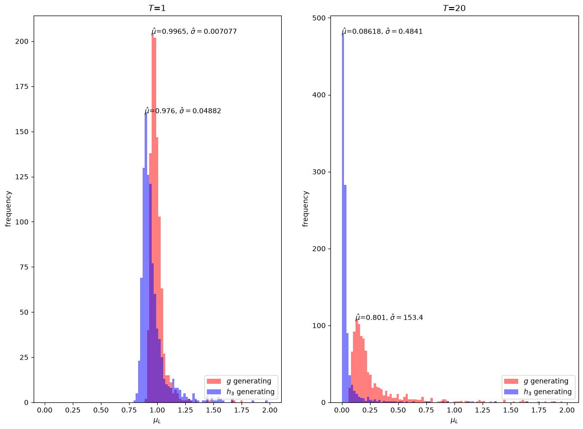
Fig. 25.7 Estimates using importance distribution \(h_3\)#
However, \(h_3\) is evidently a poor importance sampling distribution for our problem, with a mean estimate far away from \(1\) for \(T = 20\).
Notice that even at \(T = 1\), the mean estimate with importance sampling is more biased than sampling with just \(g\) itself.
Thus, our simulations suggest that for our problem we would be better off simply using Monte Carlo approximations under \(g\) than using \(h_3\) as an importance sampling distribution.